詳解目標檢測模型的評價指標及代碼實現
摘要:為了評價模型的泛化能力,即判斷模型的好壞,我們需要用某個指標來衡量,有了評價指標,就可以對比不同模型的優劣,並通過這個指標來進一步調參優化模型。
本文分享自華為雲社區《目標檢測模型的評價指標詳解及代碼實現》,作者:嵌入式視覺。
前言
為了瞭解模型的泛化能力,即判斷模型的好壞,我們需要用某個指標來衡量,有了評價指標,就可以對比不同模型的優劣,並通過這個指標來進一步調參優化模型。對於分類和迴歸兩類監督模型,分別有各自的評判標準。
不同的問題和不同的數據集都會有不同的模型評價指標,比如分類問題,數據集類別平衡的情況下可以使用準確率作為評價指標,但是現實中的數據集幾乎都是類別不平衡的,所以一般都是採用 AP 作為分類的評價指標,分別計算每個類別的 AP,再計算mAP。
一,精確率、召回率與F1
1.1,準確率
準確率(精度) – Accuracy,預測正確的結果佔總樣本的百分比,定義如下:
準確率=(TP+TN)/(TP+TN+FP+FN)
錯誤率和精度雖然常用,但是並不能滿足所有任務需求。以西瓜問題為例,假設瓜農拉來一車西瓜,我們用訓練好的模型對西瓜進行判別,現如精度只能衡量有多少比例的西瓜被我們判斷類別正確(兩類:好瓜、壞瓜)。但是若我們更加關心的是“挑出的西瓜中有多少比例是好瓜”,或者”所有好瓜中有多少比例被挑出來“,那麼精度和錯誤率這個指標顯然是不夠用的。
雖然準確率可以判斷總的正確率,但是在樣本不平衡的情況下,並不能作為很好的指標來衡量結果。舉個簡單的例子,比如在一個總樣本中,正樣本佔 90%,負樣本佔 10%,樣本是嚴重不平衡的。對於這種情況,我們只需要將全部樣本預測為正樣本即可得到 90% 的高準確率,但實際上我們並沒有很用心的分類,只是隨便無腦一分而已。這就説明了:由於樣本不平衡的問題,導致了得到的高準確率結果含有很大的水分。即如果樣本不平衡,準確率就會失效。
1.2,精確率、召回率
精確率(查準率)P、召回率(查全率)R 的計算涉及到混淆矩陣的定義,混淆矩陣表格如下:
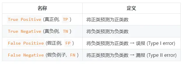
查準率與查全率計算公式:
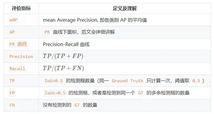
- 查準率(精確率)P=TP/(TP+FP)P=TP/(TP+FP)
- 查全率(召回率)R=TP/(TP+FN)R=TP/(TP+FN)
精準率和準確率看上去有些類似,但是完全不同的兩個概念。精準率代表對正樣本結果中的預測準確程度,而準確率則代表整體的預測準確程度,既包括正樣本,也包括負樣本。
精確率描述了模型有多準,即在預測為正例的結果中,有多少是真正例;召回率則描述了模型有多全,即在為真的樣本中,有多少被我們的模型預測為正例。精確率和召回率的區別在於分母不同,一個分母是預測為正的樣本數,另一個是原來樣本中所有的正樣本數。
1.3,F1 分數
如果想要找到 P 和 R 二者之間的一個平衡點,我們就需要一個新的指標:F1 分數。F1 分數同時考慮了查準率和查全率,讓二者同時達到最高,取一個平衡。F1 計算公式如下:
這裏的 F1 計算是針對二分類模型,多分類任務的 F1 的計算請看下面。

F1 度量的一般形式:Fβ,能讓我們表達出對查準率/查全率的偏見,Fβ 計算公式如下:

其中β>1 對查全率有更大影響,β<1 對查準率有更大影響。
不同的計算機視覺問題,對兩類錯誤有不同的偏好,常常在某一類錯誤不多於一定閾值的情況下,努力減少另一類錯誤。在目標檢測中,mAP(mean Average Precision)作為一個統一的指標將這兩種錯誤兼顧考慮。
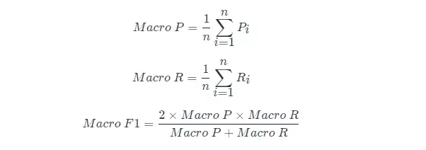
很多時候我們會有多個混淆矩陣,例如進行多次訓練/測試,每次都能得到一個混淆矩陣;或者是在多個數據集上進行訓練/測試,希望估計算法的”全局“性能;又或者是執行多分類任務,每兩兩類別的組合都對應一個混淆矩陣;…總而來説,我們希望能在 nn 個二分類混淆矩陣上綜合考慮查準率和查全率。
一種直接的做法是先在各混淆矩陣上分別計算出查準率和查全率,記為 (P1,R1),(P2,R2),...,(Pn,Rn) 然後取平均,這樣得到的是”宏查準率(Macro-P)“、”宏查準率(Macro-R)“及對應的”宏 F1F1(Macro-F1)“:
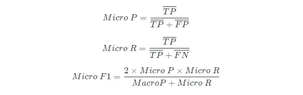
另一種做法是將各混淆矩陣對應元素進行平均,得到 TP、FP、TN、FNTP、FP、TN、FN 的平均值,再基於這些平均值計算出”微查準率“(Micro-P)、”微查全率“(Micro-R)和”微 F1“(Mairo-F1)
1.4,PR 曲線
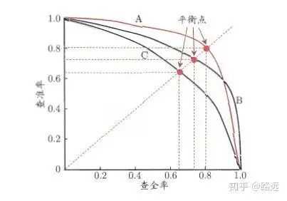
精準率和召回率的關係可以用一個 P-R 圖來展示,以查準率 P 為縱軸、查全率 R 為橫軸作圖,就得到了查準率-查全率曲線,簡稱 P-R 曲線,PR 曲線下的面積定義為 AP:
1.4.1,如何理解 P-R 曲線
可以從排序型模型或者分類模型理解。以邏輯迴歸舉例,邏輯迴歸的輸出是一個 0 到 1 之間的概率數字,因此,如果我們想要根據這個概率判斷用户好壞的話,我們就必須定義一個閾值 。通常來講,邏輯迴歸的概率越大説明越接近 1,也就可以説他是壞用户的可能性更大。比如,我們定義了閾值為 0.5,即概率小於 0.5 的我們都認為是好用户,而大於 0.5 都認為是壞用户。因此,對於閾值為 0.5 的情況下,我們可以得到相應的一對查準率和查全率。
但問題是:這個閾值是我們隨便定義的,我們並不知道這個閾值是否符合我們的要求。 因此,為了找到一個最合適的閾值滿足我們的要求,我們就必須遍歷 0 到 1 之間所有的閾值,而每個閾值下都對應着一對查準率和查全率,從而我們就得到了 PR 曲線。
最後如何找到最好的閾值點呢? 首先,需要説明的是我們對於這兩個指標的要求:我們希望查準率和查全率同時都非常高。 但實際上這兩個指標是一對矛盾體,無法做到雙高。圖中明顯看到,如果其中一個非常高,另一個肯定會非常低。選取合適的閾值點要根據實際需求,比如我們想要高的查全率,那麼我們就會犧牲一些查準率,在保證查全率最高的情況下,查準率也不那麼低。。
1.5,ROC 曲線與 AUC 面積
- PR 曲線是以 Recall 為橫軸,Precision 為縱軸;而 ROC 曲線則是以 FPR 為橫軸,TPR 為縱軸**。P-R 曲線越靠近右上角性能越好。PR 曲線的兩個指標都聚焦於正例
- PR 曲線展示的是 Precision vs Recall 的曲線,ROC 曲線展示的是 FPR(x 軸:False positive rate) vs TPR(True positive rate, TPR)曲線。
- [ ] ROC 曲線
- [ ] AUC 面積
二,AP 與 mAP
2.1,AP 與 mAP 指標理解
AP 衡量的是訓練好的模型在每個類別上的好壞,mAP 衡量的是模型在所有類別上的好壞,得到 AP 後 mAP 的計算就變得很簡單了,就是取所有 AP 的平均值。AP 的計算公式比較複雜(所以單獨作一章節內容),詳細內容參考下文。
mAP 這個術語有不同的定義。此度量指標通常用於信息檢索、圖像分類和目標檢測領域。然而這兩個領域計算 mAP 的方式卻不相同。這裏我們只談論目標檢測中的 mAP 計算方法。
mAP 常作為目標檢測算法的評價指標,具體來説就是,對於每張圖片檢測模型會輸出多個預測框(遠超真實框的個數),我們使用 IoU (Intersection Over Union,交併比)來標記預測框是否預測準確。標記完成後,隨着預測框的增多,查全率 R 總會上升,在不同查全率 R 水平下對準確率 P 做平均,即得到 AP,最後再對所有類別按其所佔比例做平均,即得到 mAP 指標。
2.2,近似計算AP
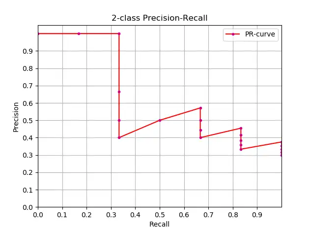
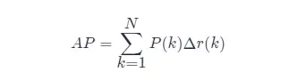
知道了AP 的定義,下一步就是理解AP計算的實現,理論上可以通過積分來計算AP,公式如下:

但通常情況下都是使用近似或者插值的方法來計算 AP。
- 近似計算 AP (approximated average precision),這種計算方式是 approximated 形式的;
- 很顯然位於一條豎直線上的點對計算 AP 沒有貢獻;
- 這裏 N 為數據總量,k 為每個樣本點的索引, Δr(k)=r(k)−r(k−1)。
近似計算 AP 和繪製 PR 曲線代碼如下:
import numpy as np
import matplotlib.pyplot as plt
class_names = ["car", "pedestrians", "bicycle"]
def draw_PR_curve(predict_scores, eval_labels, name, cls_idx=1):
 """calculate AP and draw PR curve, there are 3 types
    Parameters:
    @all_scores: single test dataset predict scores array, (-1, 3)
    @all_labels: single test dataset predict label array, (-1, 3)
    @cls_idx: the serial number of the AP to be calculated, example: 0,1,2,3...
    """
 # print('sklearn Macro-F1-Score:', f1_score(predict_scores, eval_labels, average='macro'))
 global class_names
    fig, ax = plt.subplots(nrows=1, ncols=1, figsize=(15, 10))
 # Rank the predicted scores from large to small, extract their corresponding index(index number), and generate an array
 idx = predict_scores[:, cls_idx].argsort()[::-1]
 eval_labels_descend = eval_labels[idx]
 pos_gt_num = np.sum(eval_labels == cls_idx) # number of all gt
 predict_results = np.ones_like(eval_labels)
 tp_arr = np.logical_and(predict_results == cls_idx, eval_labels_descend == cls_idx) # ndarray
 fp_arr = np.logical_and(predict_results == cls_idx, eval_labels_descend != cls_idx)
 tp_cum = np.cumsum(tp_arr).astype(float) # ndarray, Cumulative sum of array elements.
 fp_cum = np.cumsum(fp_arr).astype(float)
 precision_arr = tp_cum / (tp_cum + fp_cum) # ndarray
 recall_arr = tp_cum / pos_gt_num
    ap = 0.0
 prev_recall = 0
 for p, r in zip(precision_arr, recall_arr):
      ap += p * (r - prev_recall)
 # pdb.set_trace()
 prev_recall = r
 print("------%s, ap: %f-----" % (name, ap))
 fig_label = '[%s, %s] ap=%f' % (name, class_names[cls_idx], ap)
 ax.plot(recall_arr, precision_arr, label=fig_label)
 ax.legend(loc="lower left")
 ax.set_title("PR curve about class: %s" % (class_names[cls_idx]))
 ax.set(xticks=np.arange(0., 1, 0.05), yticks=np.arange(0., 1, 0.05))
 ax.set(xlabel="recall", ylabel="precision", xlim=[0, 1], ylim=[0, 1])
 fig.savefig("./pr-curve-%s.png" % class_names[cls_idx])
 plt.close(fig)
2.3,插值計算 AP
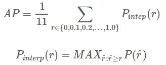
插值計算(Interpolated average precision) APAP 的公式的演變過程這裏不做討論,詳情可以參考這篇文章,我這裏的公式和圖也是參考此文章的。11 點插值計算方式計算 APAP 公式如下:
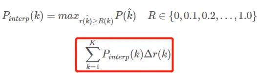
- 這是通常意義上的 11 points_Interpolated 形式的 AP,選取固定的 0,0.1,0.2,…,1.00,0.1,0.2,…,1.0 11 個閾值,這個在 PASCAL2007 中使用
- 這裏因為參與計算的只有 11 個點,所以 K=11,稱為 11 points_Interpolated,k 為閾值索引
- Pinterp(k) 取第 k 個閾值所對應的樣本點之後的樣本中的最大值,只不過這裏的閾值被限定在了 0,0.1,0.2,…,1.00,0.1,0.2,…,1.0 範圍內。
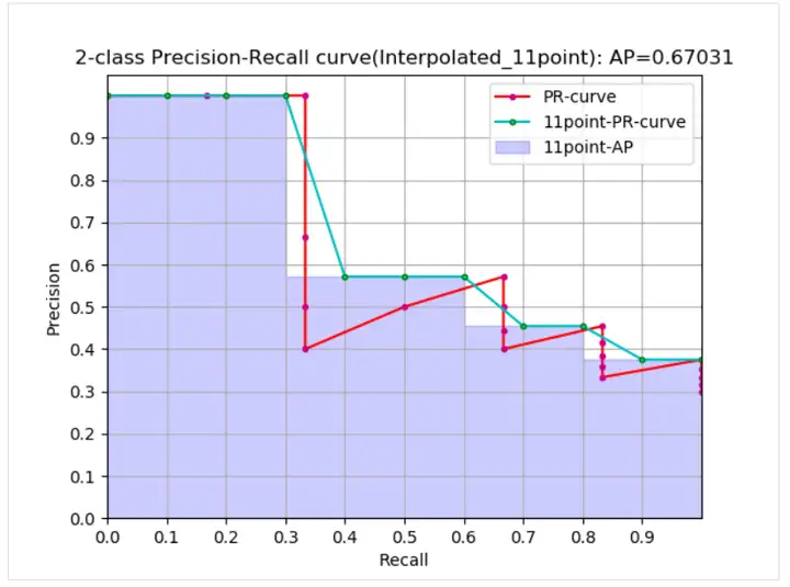
從曲線上看,真實 AP< approximated AP < Interpolated AP,11-points Interpolated AP 可能大也可能小,當數據量很多的時候會接近於 Interpolated AP,與 Interpolated AP 不同,前面的公式中計算 AP 時都是對 PR 曲線的面積估計,PASCAL 的論文裏給出的公式就更加簡單粗暴了,直接計算11 個閾值處的 precision 的平均值。PASCAL 論文給出的 11 點計算 AP 的公式如下。
1、在給定 recal 和 precision 的條件下計算 AP:
def voc_ap(rec, prec, use_07_metric=False):
 """
    ap = voc_ap(rec, prec, [use_07_metric])
    Compute VOC AP given precision and recall.
    If use_07_metric is true, uses the
    VOC 07 11 point method (default:False).
    """
 if use_07_metric:
 # 11 point metric
        ap = 0.
 for t in np.arange(0., 1.1, 0.1):
 if np.sum(rec >= t) == 0:
                p = 0
 else:
                p = np.max(prec[rec >= t])
            ap = ap + p / 11.
 else:
 # correct AP calculation
 # first append sentinel values at the end
 mrec = np.concatenate(([0.], rec, [1.]))
 mpre = np.concatenate(([0.], prec, [0.]))
 # compute the precision envelope
 for i in range(mpre.size - 1, 0, -1):
 mpre[i - 1] = np.maximum(mpre[i - 1], mpre[i])
 # to calculate area under PR curve, look for points
 # where X axis (recall) changes value
 i = np.where(mrec[1:] != mrec[:-1])[0]
 # and sum (\Delta recall) * prec
        ap = np.sum((mrec[i + 1] - mrec[i]) * mpre[i + 1])
 return ap
2、給定目標檢測結果文件和測試集標籤文件 xml 等計算 AP:
def parse_rec(filename):
 """ Parse a PASCAL VOC xml file
 Return : list, element is dict.
    """
    tree = ET.parse(filename)
    objects = []
 for obj in tree.findall('object'):
 obj_struct = {}
 obj_struct['name'] = obj.find('name').text
 obj_struct['pose'] = obj.find('pose').text
 obj_struct['truncated'] = int(obj.find('truncated').text)
 obj_struct['difficult'] = int(obj.find('difficult').text)
 bbox = obj.find('bndbox')
 obj_struct['bbox'] = [int(bbox.find('xmin').text),
 int(bbox.find('ymin').text),
 int(bbox.find('xmax').text),
 int(bbox.find('ymax').text)]
 objects.append(obj_struct)
 return objects
def voc_eval(detpath,
 annopath,
 imagesetfile,
 classname,
 cachedir,
 ovthresh=0.5,
             use_07_metric=False):
 """rec, prec, ap = voc_eval(detpath,
 annopath,
 imagesetfile,
 classname,
                                [ovthresh],
                                [use_07_metric])
    Top level function that does the PASCAL VOC evaluation.
 detpath: Path to detections result file
 detpath.format(classname) should produce the detection results file.
 annopath: Path to annotations file
 annopath.format(imagename) should be the xml annotations file.
 imagesetfile: Text file containing the list of images, one image per line.
 classname: Category name (duh)
 cachedir: Directory for caching the annotations
    [ovthresh]: Overlap threshold (default = 0.5)
    [use_07_metric]: Whether to use VOC07's 11 point AP computation
        (default False)
    """
 # assumes detections are in detpath.format(classname)
 # assumes annotations are in annopath.format(imagename)
 # assumes imagesetfile is a text file with each line an image name
 # cachedir caches the annotations in a pickle file
 # first load gt
 if not os.path.isdir(cachedir):
 os.mkdir(cachedir)
 cachefile = os.path.join(cachedir, '%s_annots.pkl' % imagesetfile)
 # read list of images
 with open(imagesetfile, 'r') as f:
        lines = f.readlines()
 imagenames = [x.strip() for x in lines]
 if not os.path.isfile(cachefile):
 # load annotations
        recs = {}
 for i, imagename in enumerate(imagenames):
            recs[imagename] = parse_rec(annopath.format(imagename))
 if i % 100 == 0:
 print('Reading annotation for {:d}/{:d}'.format(
 i + 1, len(imagenames)))
 # save
 print('Saving cached annotations to {:s}'.format(cachefile))
 with open(cachefile, 'wb') as f:
 pickle.dump(recs, f)
 else:
 # load
 with open(cachefile, 'rb') as f:
 try:
                recs = pickle.load(f)
 except:
                recs = pickle.load(f, encoding='bytes')
 # extract gt objects for this class
 class_recs = {}
 npos = 0
 for imagename in imagenames:
        R = [obj for obj in recs[imagename] if obj['name'] == classname]
 bbox = np.array([x['bbox'] for x in R])
        difficult = np.array([x['difficult'] for x in R]).astype(np.bool)
        det = [False] * len(R)
 npos = npos + sum(~difficult)
 class_recs[imagename] = {'bbox': bbox,
 'difficult': difficult,
 'det': det}
 # read dets
 detfile = detpath.format(classname)
 with open(detfile, 'r') as f:
        lines = f.readlines()
 splitlines = [x.strip().split(' ') for x in lines]
 image_ids = [x[0] for x in splitlines]
    confidence = np.array([float(x[1]) for x in splitlines])
    BB = np.array([[float(z) for z in x[2:]] for x in splitlines])
 nd = len(image_ids)
 tp = np.zeros(nd)
 fp = np.zeros(nd)
 if BB.shape[0] > 0:
 # sort by confidence
 sorted_ind = np.argsort(-confidence)
 sorted_scores = np.sort(-confidence)
        BB = BB[sorted_ind, :]
 image_ids = [image_ids[x] for x in sorted_ind]
 # go down dets and mark TPs and FPs
 for d in range(nd):
            R = class_recs[image_ids[d]]
            bb = BB[d, :].astype(float)
 ovmax = -np.inf
            BBGT = R['bbox'].astype(float)
 if BBGT.size > 0:
 # compute overlaps
 # intersection
 ixmin = np.maximum(BBGT[:, 0], bb[0])
 iymin = np.maximum(BBGT[:, 1], bb[1])
 ixmax = np.minimum(BBGT[:, 2], bb[2])
 iymax = np.minimum(BBGT[:, 3], bb[3])
 iw = np.maximum(ixmax - ixmin + 1., 0.)
 ih = np.maximum(iymax - iymin + 1., 0.)
                inters = iw * ih
 # union
 uni = ((bb[2] - bb[0] + 1.) * (bb[3] - bb[1] + 1.) +
 (BBGT[:, 2] - BBGT[:, 0] + 1.) *
 (BBGT[:, 3] - BBGT[:, 1] + 1.) - inters)
                overlaps = inters / uni
 ovmax = np.max(overlaps)
 jmax = np.argmax(overlaps)
 if ovmax > ovthresh:
 if not R['difficult'][jmax]:
 if not R['det'][jmax]:
 tp[d] = 1.
                        R['det'][jmax] = 1
 else:
 fp[d] = 1.
 else:
 fp[d] = 1.
 # compute precision recall
 fp = np.cumsum(fp)
 tp = np.cumsum(tp)
    rec = tp / float(npos)
 # avoid divide by zero in case the first detection matches a difficult
 # ground truth
 prec = tp / np.maximum(tp + fp, np.finfo(np.float64).eps)
    ap = voc_ap(rec, prec, use_07_metric)
 return rec, prec, ap
2.4,mAP 計算方法
因為 mAP 值的計算是對數據集中所有類別的 AP 值求平均,所以我們要計算 mAP,首先得知道某一類別的 AP 值怎麼求。不同數據集的某類別的 AP 計算方法大同小異,主要分為三種:
(1)在 VOC2007,只需要選取當 Recall>=0,0.1,0.2,...,1Recall>=0,0.1,0.2,...,1 共 11 個點時的 Precision 最大值,然後 APAP 就是這 11 個 Precision 的平均值,mAPmAP 就是所有類別 APAP 值的平均。VOC 數據集中計算 APAP 的代碼(用的是插值計算方法,代碼出自py-faster-rcnn倉庫)
(2)在 VOC2010 及以後,需要針對每一個不同的 Recall 值(包括 0 和 1),選取其大於等於這些 Recall 值時的 Precision 最大值,然後計算 PR 曲線下面積作為 AP 值,mAPmAP 就是所有類別 AP 值的平均。
(3)COCO 數據集,設定多個 IOU 閾值(0.5-0.95, 0.05 為步長),在每一個 IOU 閾值下都有某一類別的 AP 值,然後求不同 IOU 閾值下的 AP 平均,就是所求的最終的某類別的 AP 值。
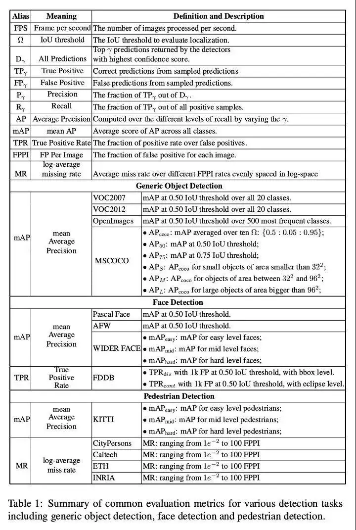
三,目標檢測度量標準彙總
四,參考資料
- 目標檢測評價標準-AP mAP
- 目標檢測的性能評價指標
- Soft-NMS
- Recent Advances in Deep Learning for Object Detection
- A Simple and Fast Implementation of Faster R-CNN
- 分類模型評估指標——準確率、精準率、召回率、F1、ROC曲線、AUC曲線
- 一文讓你徹底理解準確率,精準率,召回率,真正率,假正率,ROC/AUC
- 使用卷積神經網絡實現圖片去摩爾紋
- 內核不中斷前提下,Gaussdb(DWS)內存報錯排查方法
- 簡述幾種常用的排序算法
- 自動調優工具AOE,讓你的模型在昇騰平台上高效運行
- GaussDB(DWS)運維:導致SQL執行不下推的改寫方案
- 詳解目標檢測模型的評價指標及代碼實現
- CosineWarmup理論與代碼實戰
- 淺談DWS函數出參方式
- 代碼實戰帶你瞭解深度學習中的混合精度訓練
- python進階:帶你學習實時目標跟蹤
- Ascend CL兩種數據預處理的方式:AIPP和DVPP
- 詳解ResNet 網絡,如何讓網絡變得更“深”了
- 帶你掌握如何查看並讀懂昇騰平台的應用日誌
- InstructPix2Pix: 動動嘴皮子,超越PS
- 何為神經網絡卷積層?
- 在昇騰平台上對TensorFlow網絡進行性能調優
- 介紹3種ssh遠程連接的方式
- 分佈式數據庫架構路線大揭祕
- DBA必備的Mysql知識點:數據類型和運算符
- 5個高併發導致數倉資源類報錯分析